Classification task 27 Feb 2019
This notebook contains steps and code to get started with classification tasks. We wil be using the Fashin-MNIST dataset, an alternative dataset to the well-known MNIST dataset
Setup
This cell contains code for referring the common imports that we will be using through this notebook.
# Common imports
import numpy as np
import os

# to make this notebook's output stable across runs
np.random.seed(10)

# To plot pretty figures
import matplotlib as mpl
import matplotlib.pyplot as plt
mpl.rc('axes', labelsize=14)
mpl.rc('xtick', labelsize=12)
mpl.rc('ytick', labelsize=12)
Fashion-MNIST Dataset
Fashion-MNIST is a dataset of Zalando’s article images, consisting of a training set of 60,000 examples and a test set of 10,000 examples. Each example is a 28x28 grayscale image, associated with a label from 10 classes.
- 0 T-shirt/top
- 1 Trouser
- 2 Pullover
- 3 Dress
- 4 Coat
- 5 Sandal
- 6 Shirt
- 7 Sneaker
- 8 Bag
- 9 Ankle boot
We will be using openml, a popular library that makes interesting datasets available.
# Fetching the Fashion-MNIST dataset by using openml
from sklearn.datasets import fetch_openml
mnist = fetch_openml('Fashion-MNIST', version=1, cache=True)
mnist.target = mnist.target.astype(np.int8) # fetch_openml() returns targets as strings
mnist["data"], mnist["target"]
(array([[0., 0., 0., ..., 0., 0., 0.],
        [0., 0., 0., ..., 0., 0., 0.],
        [0., 0., 0., ..., 0., 0., 0.],
        ...,
        [0., 0., 0., ..., 0., 0., 0.],
        [0., 0., 0., ..., 0., 0., 0.],
        [0., 0., 0., ..., 0., 0., 0.]]),
 array([9, 0, 0, ..., 8, 1, 5], dtype=int8))
# Let's figure out how many instance our dataset contains
mnist.data.shape
(70000, 784)
# Assign features to "X", and labels to "y"
X, y = mnist["data"], mnist["target"]
X.shape, y.shape
((70000, 784), (70000,))
# Pick up an item and show it
item = X[36030]
item_image = item.reshape(28, 28)
plt.imshow(item_image, cmap = mpl.cm.binary, interpolation="nearest")
plt.axis("off")
plt.show()
y[36030]
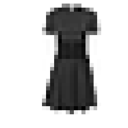
3
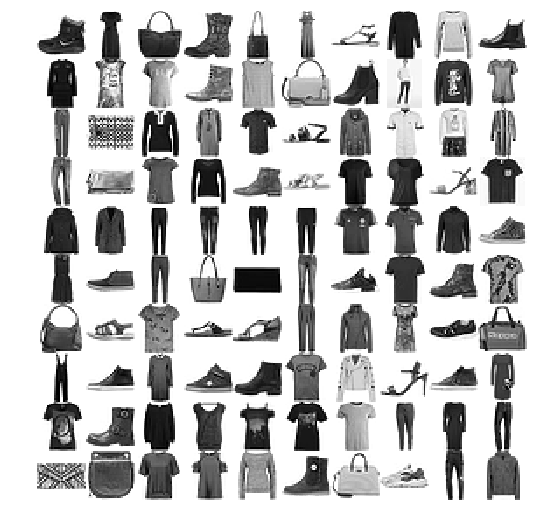
Explore data
The following cells contain code to plot a portion of the data. The idea is getting familiar with the data by visualizing it.
# Create a function to plot items
def plot_items(instances, images_per_row=10, **options):
    size = 28
    images_per_row = min(len(instances), images_per_row)
    images = [instance.reshape(size,size) for instance in instances]
    n_rows = (len(instances) - 1) // images_per_row + 1
    row_images = []
    n_empty = n_rows * images_per_row - len(instances)
    images.append(np.zeros((size, size * n_empty)))
    for row in range(n_rows):
        rimages = images[row * images_per_row : (row + 1) * images_per_row]
        row_images.append(np.concatenate(rimages, axis=1))
    image = np.concatenate(row_images, axis=0)
    plt.imshow(image, cmap = mpl.cm.binary, **options)
    plt.axis("off")
# Show a batch of items.
plt.figure(figsize=(9,9))
example_images = np.r_[X[:2500:50], X[30000:35000:100]]
plot_items(example_images, images_per_row=10)
plt.show()
Split the data into train and test dataset
These cells contain two alternatives for splitting the dataset into train and test dataset. While the first code one assumes that data is randomly distributed, the second one includes a step to randomly distribute the test data.
X_train, X_test, y_train, y_test = X[:60000], X[60000:], y[:60000], y[60000:]
import numpy as np

shuffle_index = np.random.permutation(60000)
X_train, y_train = X_train[shuffle_index], y_train[shuffle_index]
Binary Classifier
Our first task will be to build a binary classifier that predicts if a item is a dress or not (We could have picked up another item). By re labeling the data into these two classes (if dress or not), we are obtaining a skewed dataset. That is, there is not balance in the number of intances per each class.
y_train_dress = (y_train == 3)
y_test_dress = (y_test == 3)
# Train a SGDClassifier
from sklearn.linear_model import SGDClassifier

sgd_clf = SGDClassifier(max_iter=5, tol=-np.infty, random_state=10)
sgd_clf.fit(X_train, y_train_dress)
SGDClassifier(alpha=0.0001, average=False, class_weight=None,
       early_stopping=False, epsilon=0.1, eta0=0.0, fit_intercept=True,
       l1_ratio=0.15, learning_rate='optimal', loss='hinge', max_iter=5,
       n_iter=None, n_iter_no_change=5, n_jobs=None, penalty='l2',
       power_t=0.5, random_state=10, shuffle=True, tol=-inf,
       validation_fraction=0.1, verbose=0, warm_start=False)
# Once fitting our model, we can predict the result for a specific instance
sgd_clf.predict([item])
array([ True])
Measuring accuracy using Cross Validation
Cross Validation is a popular technique to estimate perfomance measures but for validation sets. The idea is to obtain measures that leads us to understand the possible performance in unseen data.
from sklearn.model_selection import cross_val_score
cross_val_score(sgd_clf, X_train, y_train_dress, cv=3, scoring="accuracy")
array([0.96185, 0.9571 , 0.9612 ])
The following code helps to understand what is going on behind the scenes when we use cross validation.
from sklearn.model_selection import StratifiedKFold
from sklearn.base import clone

skfolds = StratifiedKFold(n_splits=3, random_state=10)

for train_index, val_index in skfolds.split(X_train, y_train_dress):
    clone_clf = clone(sgd_clf)
    X_train_folds = X_train[train_index]
    y_train_folds = (y_train_dress[train_index])
    X_val_fold = X_train[val_index]
    y_val_fold = (y_train_dress[val_index])

    clone_clf.fit(X_train_folds, y_train_folds)
    y_pred = clone_clf.predict(X_val_fold)
    n_correct = sum(y_pred == y_val_fold)
    print(n_correct / len(y_pred))
0.96185
0.9571
0.9612
The accuracy obtained is pretty atractive, being this a first attempt. However, sometimes just paying attention to the accuracy can be misleading. In the following lines, a naive NeverDressClassifier can obtain 90% of accuracy
from sklearn.base import BaseEstimator
class NeverDressClassifier(BaseEstimator):
    def fit(self, X, y=None):
        pass
    def predict(self, X):
        return np.zeros((len(X), 1), dtype=bool)
never_dress_clf = NeverDressClassifier()
cross_val_score(never_dress_clf, X_train, y_train_dress,
                cv=3, scoring="accuracy")
array([0.9029 , 0.89605, 0.90105])
Confusion Matrix
The confusion matrix provides more information about the performance of a classifier and allow us to build other important metrics in classification tasks. This matrix contrast the actual label against the precited label in the following way:
| ____ | Predicted Neg. | Predicted Pos. |
|---|---|---|
| Actual Neg. | TN | FP |
| Actual Pos. | FN | TP |
Where:
TN: True Negative
TP: True Positive
FP: False Positive
FN: False Negative
# Obtain predictions by using the SGDClassifier and Cross Validation
from sklearn.model_selection import cross_val_predict
y_train_pred = cross_val_predict(sgd_clf, X_train, y_train_dress, cv=3)
from sklearn.metrics import confusion_matrix
confusion_matrix(y_train_dress, y_train_pred)
array([[53176,   824],
       [ 1573,  4427]], dtype=int64)
The false positive and false negative values give us suplemental information to understand the performance of our model. An ideal model will show zero for these two values, as the following cells show.
y_train_perfect_predictions = y_train_dress
confusion_matrix(y_train_dress, y_train_perfect_predictions)
array([[54000,     0],
       [    0,  6000]], dtype=int64)
Precision and Recall
Precision and Recall are two measures that together give more information than the accuracy does. They are defined in the following way:
Precision = TP / (TP + FP)
Recall = TP / (TP + FN)
We can obtain them by using utilities or by calculation.
from sklearn.metrics import precision_score, recall_score
precision_score(y_train_dress, y_train_pred)
0.8430775090458961
4427 / (4427 + 824) # TP / (TP + FP)
0.8430775090458961
recall_score(y_train_dress, y_train_pred)
0.7378333333333333
4427 / (4427 + 1573) # TP / (TP + FN)
0.7378333333333333
Precision a recall together provide more information than the accuracy does, but there is one score called F1 score, that merges the precision and recall to give us one idea of the performance of the model. A greater F1 score (close to 1) is better. It is defined in the following way:
f1_score= 2 (Precision)(Recall) / (Precision + Recall)
from sklearn.metrics import f1_score
f1_score(y_train_dress, y_train_pred)
0.7869522709092526
Precision/Recall tradeoff
Although precision and recall closing to one are better values, there is tradeoff between these two metrics. That is, for a specific trained model, if we modified the threshold we might obtain a better precision but a worse recall and viceversa.
# For our item, obtain the score that leads to its classification
y_scores = sgd_clf.decision_function([item])
y_scores
array([373576.68954112])
# Compute the prediction with a threshold of zero
threshold = 0
y_item_pred = (y_scores > threshold)
y_item_pred
array([ True])
# Compute the prediction with a different threshold
threshold = 500000
y_item_pred = (y_scores > threshold)
y_item_pred
array([False])
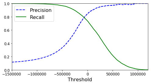
As we see, by modifiying the threshold we might alter the prediction. Now, let’s show how the precision and recall change as a function of the threshold
# Obtain the scores for each instance by using SGDC and cross validation
y_scores = cross_val_predict(sgd_clf, X_train, y_train_dress, cv=3,
                             method="decision_function")
# Generate the precision and recall values for a range of thresholds
from sklearn.metrics import precision_recall_curve
precisions, recalls, thresholds = precision_recall_curve(y_train_dress,
                                                         y_scores)
# Plot the precision and recall as a function of the threshold
def plot_precision_recall_vs_threshold(precisions, recalls, thresholds):
    plt.plot(thresholds, precisions[:-1], "b--", label="Precision", linewidth=2)
    plt.plot(thresholds, recalls[:-1], "g-", label="Recall", linewidth=2)
    plt.xlabel("Threshold", fontsize=16)
    plt.legend(loc="upper left", fontsize=16)
    plt.ylim([0, 1])

plt.figure(figsize=(8, 4))
plot_precision_recall_vs_threshold(precisions, recalls, thresholds)
plt.xlim([-1500000, 1200000])
plt.show()
(y_train_pred == (y_scores > 0)).all()
True
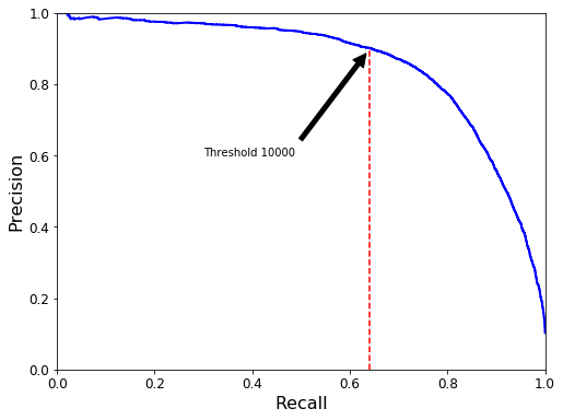
By setting up a threshold = 0, we obtain our original prediction with a precision rate of 84%. However, if we use another threshold, we can obtain a better precision but at the expense of worse recall.
y_train_pred_90 = (y_scores > 100000)
precision_score(y_train_dress, y_train_pred_90)
0.9000935891436593
recall_score(y_train_dress, y_train_pred_90)
0.6411666666666667
def plot_precision_vs_recall(precisions, recalls):
    plt.plot(recalls, precisions, "b-", linewidth=2)
    plt.xlabel("Recall", fontsize=16)
    plt.ylabel("Precision", fontsize=16)
    plt.axis([0, 1, 0, 1])

plt.figure(figsize=(8, 6))
plot_precision_vs_recall(precisions, recalls)
plt.annotate('Threshold 10000', xy=(0.641, 0.90), xytext=(0.3, 0.6),
             arrowprops=dict(facecolor='black', shrink=0.05),
             )

plt.plot([0.641, 0.641], [0, 0.9], "r--")

plt.show()
ROC Curves
The receiver operating characteristic (ROC) curve is commonly used for classification tasks too. Unlike the precision-recall curve, the ROC curve plots the TPR: True Positive Rate (Recall) against the FPR: False Positive Rate. The FPR is defined as the ratio of negative instances that are missclassified as positives. The FPR is equal to one minus the TNR: True Negative Rate also known as Specifity.
from sklearn.metrics import roc_curve
# TPR: True Positive Rate
# FPR: False Positive Rate
fpr, tpr, thresholds = roc_curve(y_train_dress, y_scores)
def plot_roc_curve(fpr, tpr, label=None):
    plt.plot(fpr, tpr, linewidth=2, label=label)
    plt.plot([0, 1], [0, 1], 'k--')
    plt.axis([0, 1, 0, 1])
    plt.xlabel('False Positive Rate', fontsize=16)
    plt.ylabel('True Positive Rate', fontsize=16)

plt.figure(figsize=(8, 6))
plot_roc_curve(fpr, tpr)
plt.show()
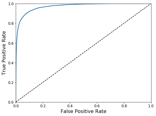
The area under curve is commonly used to compare different models. An area closer to one is better.
from sklearn.metrics import roc_auc_score
roc_auc_score(y_train_dress, y_scores)
0.9708191851851852
Let’s train another model and then compare it to our previous model.
from sklearn.ensemble import RandomForestClassifier
forest_clf = RandomForestClassifier(n_estimators=10, random_state=10)
y_probas_forest = cross_val_predict(forest_clf, X_train, y_train_dress, cv=3,
                                    method="predict_proba")
y_scores_forest = y_probas_forest[:, 1] # score = proba of positive class
fpr_forest, tpr_forest, thresholds_forest = roc_curve(
    y_train_dress,y_scores_forest)
plt.figure(figsize=(8, 6))
plt.plot(fpr, tpr, "b:", linewidth=2, label="SGD")
plot_roc_curve(fpr_forest, tpr_forest, "Random Forest")
plt.legend(loc="lower right", fontsize=16)
plt.show()
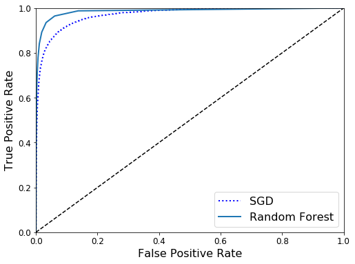
roc_auc_score(y_train_dress, y_scores_forest)
0.9857603503086421
y_train_pred_forest = cross_val_predict(forest_clf, X_train, y_train_dress, cv=3)
precision_score(y_train_dress, y_train_pred_forest)
0.9294515103338633
recall_score(y_train_dress, y_train_pred_forest)
0.7795
Multiclass classification
In this section, we introduce multiclass classifiers in order to predict one of the ten classes of our dataset. Recall our 10 classes:
0 T-shirt/top
1 Trouser
2 Pullover
3 Dress
4 Coat
5 Sandal
6 Shirt
7 Sneaker
8 Bag
9 Ankle boot
# Fir the SGDClassifier with our "y" containing 10 classes
sgd_clf.fit(X_train, y_train)
sgd_clf.predict([item])
array([3], dtype=int8)
# Obtain the scores for our selected item
item_scores = sgd_clf.decision_function([item])
item_scores
array([[ -567587.25968507,  -396720.40311972,  -798576.1395802 ,
          373576.68954112,  -636013.02740982, -2174210.81529276,
         -481888.83230268, -1360399.01950886,  -889621.21801326,
         -880520.24583804]])
See that our fitted model yields scores as an vector 1 x 10. Since our item is represented by label number 3, the index 3 of the scores yields the highest value.
np.argmax(item_scores)
3
sgd_clf.classes_
array([0, 1, 2, 3, 4, 5, 6, 7, 8, 9], dtype=int8)
sgd_clf.classes_[3]
3
By Default, the SGDClassifier takes advantage of the OneVsAll strategy in order to obtain a multiclass classification from a binary classification. However, we can use the OneVsOne strategy for this specific classifier. When we do that, a total of 45 = (10)(10 -1)/2 will be trained.
from sklearn.multiclass import OneVsOneClassifier
ovo_clf = OneVsOneClassifier(SGDClassifier(max_iter=5, tol=-np.infty, random_state=10))
ovo_clf.fit(X_train, y_train)
ovo_clf.predict([item])
array([3], dtype=int8)
len(ovo_clf.estimators_)
45
forest_clf.fit(X_train, y_train)
forest_clf.predict([item])  # or item.reshape(1, -1)
array([3], dtype=int8)
forest_clf.predict_proba([item])
array([[0., 0., 0., 1., 0., 0., 0., 0., 0., 0.]])
cross_val_score(sgd_clf, X_train, y_train, cv=3, scoring="accuracy")
array([0.781 , 0.74295, 0.7822 ])
The accuracy of our trained model can be improved by applying standar scaling to the the data.
from sklearn.preprocessing import StandardScaler
scaler = StandardScaler()
X_train_scaled = scaler.fit_transform(X_train.astype(np.float64))
cross_val_score(sgd_clf, X_train_scaled, y_train, cv=3, scoring="accuracy")
array([0.82845, 0.8244 , 0.8343 ])
Error Analysis
Like the confusion matrix used in a binary classificatin task, we can obtain and plot a confusion matrix for a multiclass classification.
y_train_pred = cross_val_predict(sgd_clf, X_train_scaled, y_train, cv=3)
conf_mx = confusion_matrix(y_train, y_train_pred)
conf_mx
array([[4998,   10,  128,  401,   20,    2,  339,    0,  102,    0],
       [  12, 5715,   53,  173,   13,    1,   30,    0,    3,    0],
       [  47,    4, 4640,  112,  743,    1,  362,    1,   89,    1],
       [ 270,   81,   98, 5245,  178,    0,  110,    0,   17,    1],
       [  17,    4, 1066,  397, 4104,    1,  378,    1,   31,    1],
       [   5,    1,    2,    7,    0, 5636,    6,  162,   57,  124],
       [1014,   19,  929,  400,  606,    0, 2826,    3,  202,    1],
       [   0,    0,    0,    0,    0,  467,    1, 5288,   15,  229],
       [  39,    2,   38,  120,   31,   18,   70,   33, 5642,    7],
       [   0,    3,    0,    4,    0,  125,    1,  214,    4, 5649]],
      dtype=int64)
def plot_confusion_matrix(matrix):
    fig = plt.figure(figsize=(8,8))
    ax = fig.add_subplot(111)
    cax = ax.matshow(matrix)
    fig.colorbar(cax)
plt.matshow(conf_mx, cmap=plt.cm.gray)
plt.show()
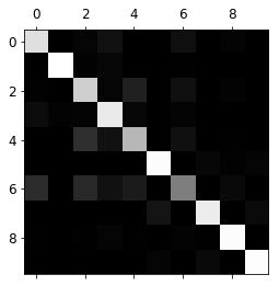
Thi intensity on the diagonal gives us an idea of the accuracy, while the intensity on other squares gives us an idea of missclassification. In order to pay attention to missclassifications we can normalize those values and set the diagonal to zero.
row_sums = conf_mx.sum(axis=1, keepdims=True)
norm_conf_mx = conf_mx / row_sums
# *** Document fill_diagonal
np.fill_diagonal(norm_conf_mx, 0)
plt.matshow(norm_conf_mx, cmap=plt.cm.gray)
plt.show()
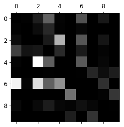
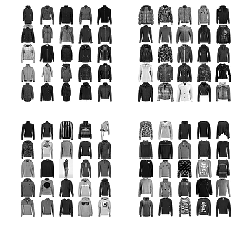
cl_a, cl_b = 4, 2
# 4 Coat
# 2 Pullover
X_aa = X_train[(y_train == cl_a) & (y_train_pred == cl_a)]
X_ab = X_train[(y_train == cl_a) & (y_train_pred == cl_b)]
X_ba = X_train[(y_train == cl_b) & (y_train_pred == cl_a)]
X_bb = X_train[(y_train == cl_b) & (y_train_pred == cl_b)]

plt.figure(figsize=(8,8))
plt.subplot(221); plot_items(X_aa[:25], images_per_row=5)
plt.subplot(222); plot_items(X_ab[:25], images_per_row=5)
plt.subplot(223); plot_items(X_ba[:25], images_per_row=5)
plt.subplot(224); plot_items(X_bb[:25], images_per_row=5)
plt.show()
Multilabel Classification
Mutilabel classification consists of assigning more than one label to a specific instance. To put this into practice, let’s create two labels for each specific instance, Men (M), Women(W).
from sklearn.neighbors import KNeighborsClassifier

# - 0 T-shirt/top -> W/M
# - 1 Trouser -> W/M
# - 2 Pullover -> W/M
# - 3 Dress -> W
# - 4 Coat -> W/M
# - 5 Sandal -> W/M
# - 6 Shirt -> M
# - 7 Sneaker -> W/M
# - 8 Bag ->
# - 9 Ankle boot -> W

y_train_w = np.isin(y_train, [0,1,2,3,4,5,7,9])
y_train_m = np.isin(y_train, [0,1,2,4,5,6,7])
y_multilabel = np.c_[y_train_w, y_train_m]

knn_clf = KNeighborsClassifier()
knn_clf.fit(X_train, y_multilabel)
KNeighborsClassifier(algorithm='auto', leaf_size=30, metric='minkowski',
           metric_params=None, n_jobs=None, n_neighbors=5, p=2,
           weights='uniform')
# Recall that our item is a dress
knn_clf.predict([item])
array([[ True, False]])
y_train_knn_pred = cross_val_predict(knn_clf, X_train, y_multilabel, cv=3, n_jobs=-1)
f1_score(y_multilabel, y_train_knn_pred, average="macro")
0.9612839736578104
References
- Hands-On Machine Learning with Scikit-Learn and TensorFlow: Concepts, Tools, and Techniques to Build Intelligent Systems