Training Linear Regression Models 22 Mar 2019
In this notebook, we will review some techniques for training a linear regression model.
Setup
This cell contains code for referring the common imports that we will be using through this notebook.
# Common imports
import numpy as np
import os

# to make this notebook's output stable across runs
np.random.seed(10)

# To plot pretty figures
import matplotlib as mpl
import matplotlib.pyplot as plt
mpl.rc('axes', labelsize=14)
mpl.rc('xtick', labelsize=12)
mpl.rc('ytick', labelsize=12)
Linear regression using the Normal Equation
Recall that we can obtain the theta parameters by the direct normal equation.
theta = (XT.X)-1 . XT . y
Let’s simulate some dataset (with just one feature) and a linear form.
import numpy as np
m =100 # m: number of data points
n = 1 # n: number of features

X_i = 2 * np.random.rand(m, 1)
y = 1 + 4 * X_i + np.random.randn(m, 1)
plt.plot(X_i, y, "b.")
plt.xlabel("$x_1$", fontsize=18)
plt.ylabel("$y$", rotation=0, fontsize=18)
plt.axis([0, 2, -2, 12])
plt.show()
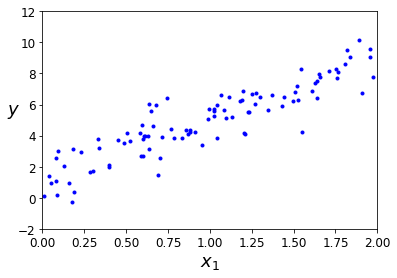
In order to operate the normal equation, we need that X contain an aditional one column vector for the bias term “b” (y = theta1 * x + b)
X = np.c_[np.ones((m, 1)), X_i]  # add x0 = 1 to each instance
theta = np.linalg.inv(X.T.dot(X)).dot(X.T).dot(y)
theta
array([[1.24963579],
       [3.81740108]])
So, we have obtained the theta values theta0(=b: bias term) and theta 1 by using the normal equation. Now, we can make predictions for new input values.
X_i_new = np.array([[0], [2]])
X_new = np.c_[np.ones((2, 1)), X_i_new]  # add x0 = 1 to each instance
y_predict = X_new.dot(theta)
y_predict
array([[1.24963579],
       [8.88443794]])
By having a couple of predictions, we can plot our linear hyphotesis (A line just need two points to be defined, so plottable)
plt.plot(X_i_new, y_predict, "r-", label="Prediction")
plt.plot(X_i, y, "b.")
plt.xlabel("$x_1$", fontsize=18)
plt.ylabel("$y$", rotation=0, fontsize=18)
plt.legend(loc="upper left", fontsize=14)
plt.axis([0, 2, -2, 12])
plt.show()

Linear Regression using the sklearn
When we use LinearRegression from sklearn we do not need to add the one column vector for the bias term.
from sklearn.linear_model import LinearRegression
lin_reg = LinearRegression()
lin_reg.fit(X_i, y)
lin_reg.intercept_, lin_reg.coef_
(array([1.24963579]), array([[3.81740108]]))
lin_reg.predict(X_i_new)
array([[1.24963579],
       [8.88443794]])
The LinearRegression class is based on the scipy.linalg.lstsq() function (the name stands for “least squares”). So, we might obtain the parameters directly by calling this function. Notice that results are the same.
theta_svd, residuals, rank, s = np.linalg.lstsq(X, y, rcond=1e-6)
theta_svd
array([[1.24963579],
       [3.81740108]])
Another way to obtain the theta parameters is by using the pseudoinverse of X (specifically the Moore-Penrose inverse)
np.linalg.pinv(X).dot(y)
array([[1.24963579],
       [3.81740108]])
Linear Regression using batch gradient descent
Gradient descent is an algorithm applied not only to linear regression but also to other models. In linear regression is works pretty well even when n (number of features) is high and even greater than m (number of data points).
alpha = 0.1
iterations = 1000
# m: number of data points
# n: number of features
theta = np.random.randn(n + 1, 1) # random initialization

for iteration in range(iterations):
    theta_grad = 1/m * X.T.dot(X.dot(theta) - y)
    theta = theta -  alpha * theta_grad

theta
array([[1.24963654],
       [3.81740041]])
As we see, by using batch gradient descent, we obtained theta parameters that are equal to theta parameters previously obtained. We can use these theta parameters to predit y for a new X.
X_new.dot(theta)
array([[1.24963654],
       [8.88443737]])
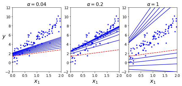
The alpha hyperparameter used is also known as learning rate. This value plays an important role in the process of learning (obtaining theta values). On one hand a small value of alpha causes a slow learning process, on the other hand a large value of alpha might cause that the gradient descent algorithm does not converge to unique theta parameters. The following cells show how the alpha values influence the learning process.
theta_path_bgd = []

def plot_gradient_descent(theta, alpha, theta_path=None):
    m = len(X)
    plt.plot(X_i, y, "b.")
    iterations = 1000
    for iteration in range(iterations):
        if iteration < 10:
            y_predict = X_new.dot(theta)
            style = "b-" if iteration > 0 else "r--"
            plt.plot(X_i_new, y_predict, style)
        theta_grad = 1/m * X.T.dot(X.dot(theta) - y)
        theta = theta - alpha * theta_grad
        if theta_path is not None:
            theta_path.append(theta)
    plt.xlabel("$x_1$", fontsize=18)
    plt.axis([0, 2, -2, 12])
    plt.title(r"$\alpha = {}$".format(alpha), fontsize=16)
np.random.seed(10)
theta = np.random.randn(n + 1,1)  # random initialization

plt.figure(figsize=(10,4))
plt.subplot(131); plot_gradient_descent(theta, alpha=0.04)
plt.ylabel("$y$", rotation=0, fontsize=18)
plt.subplot(132); plot_gradient_descent(theta, alpha=0.2, theta_path=theta_path_bgd)
plt.subplot(133); plot_gradient_descent(theta, alpha=1)

plt.show()
Stochastic Gradient Descent
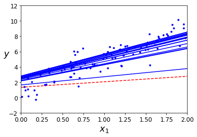
For large datasets (large m value), calculating the theta parameters using batch gradient descent might be computationally expensive. An alternative to batch gradient descent is stochastic gradient descent that uses just one data point in each iteration. As a result, the theta parameters for some data points might walk away from the global optima, but in average they tend to get closer.
theta_path_sgd = []
m = len(X)
n = 1
np.random.seed(10)
epochs = 50
c1, c2 = 5, 50  # learning schedule hyperparameters

def learning_schedule(c):
    return c1 / (c + c2)

theta = np.random.randn(n + 1,1)  # random initialization

for epoch in range(epochs):
    for i in range(m):
        if epoch == 0 and i < 20:
            y_predict = X_new.dot(theta)
            style = "b-" if i > 0 else "r--"
            plt.plot(X_i_new, y_predict, style)
        random_index = np.random.randint(m)
        xi = X[random_index:random_index+1]
        yi = y[random_index:random_index+1]
        theta_grad = xi.T.dot(xi.dot(theta) - yi)
        alpha = learning_schedule(epoch * m + i)
        theta = theta - alpha * theta_grad
        theta_path_sgd.append(theta)

plt.plot(X_i, y, "b.")
plt.xlabel("$x_1$", fontsize=18)
plt.ylabel("$y$", rotation=0, fontsize=18)
plt.axis([0, 2, -2, 12])
plt.show()
theta
array([[1.28074794],
       [3.81397122]])
As we see, we obtain theta parameters pretty close to the optimal values, but they are no as good as those obtained by batch gradient desdent.
In the following celles, we use the sklearn library to apply Stochastic Gradient Descent to our dataset.
from sklearn.linear_model import SGDRegressor
sgd_reg = SGDRegressor(max_iter=50, tol=-np.infty, penalty=None, eta0=0.1, random_state=10)
sgd_reg.fit(X_i, y.ravel())
SGDRegressor(alpha=0.0001, average=False, early_stopping=False, epsilon=0.1,
       eta0=0.1, fit_intercept=True, l1_ratio=0.15,
       learning_rate='invscaling', loss='squared_loss', max_iter=50,
       n_iter=None, n_iter_no_change=5, penalty=None, power_t=0.25,
       random_state=10, shuffle=True, tol=-inf, validation_fraction=0.1,
       verbose=0, warm_start=False)
sgd_reg.intercept_, sgd_reg.coef_
(array([1.25297573]), array([3.8154958]))
Mini-batch gradient descent
A reasonable alternative to the two previous algorithms is mini-batch gradient descent. The idea is to calculate the gradients on a subset of data points (mini-batch).
theta_path_mgd = []

iterations = 100
minibatch_size = 20

np.random.seed(10)
theta = np.random.randn(2,1)  # random initialization

c1, c2 = 200, 1000
def learning_schedule(c):
    return c1 / (c + c2)

c = 0
for epoch in range(iterations):
    shuffled_indices = np.random.permutation(m)
    X_shuffled = X[shuffled_indices]
    y_shuffled = y[shuffled_indices]
    for i in range(0, m, minibatch_size):
        c += 1
        xi = X_shuffled[i:i+minibatch_size]
        yi = y_shuffled[i:i+minibatch_size]
        theta_grad = 1/minibatch_size * xi.T.dot(xi.dot(theta) - yi)
        alpha = learning_schedule(c)
        theta = theta - alpha * theta_grad
        theta_path_mgd.append(theta)
theta
array([[1.23674364],
       [3.80289025]])
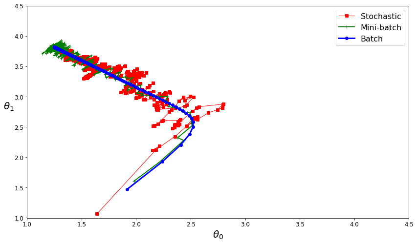
Now we can show how these three algorithms reach o get closer to the global optimal parameters.
theta_path_bgd = np.array(theta_path_bgd)
theta_path_sgd = np.array(theta_path_sgd)
theta_path_mgd = np.array(theta_path_mgd)
plt.figure(figsize=(14,8))
plt.plot(theta_path_sgd[:, 0], theta_path_sgd[:, 1], "r-s", linewidth=1, label="Stochastic")
plt.plot(theta_path_mgd[:, 0], theta_path_mgd[:, 1], "g-+", linewidth=2, label="Mini-batch")
plt.plot(theta_path_bgd[:, 0], theta_path_bgd[:, 1], "b-o", linewidth=3, label="Batch")
plt.legend(loc="upper right", fontsize=16)
plt.xlabel(r"$\theta_0$", fontsize=20)
plt.ylabel(r"$\theta_1$   ", fontsize=20, rotation=0)
plt.axis([1, 4.5, 1, 4.5])
plt.show()
Polynomial Regression
Polynomial regression allows us to increase the flexibility of our linear hyphotesis by generating features based on the polynomial calculations of the given features. In the following example, we create a second feature by squaring a given input of one just feature.
import numpy as np
import numpy.random as rnd

np.random.seed(10)
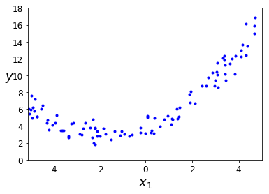
Let’s simulate a cuadratic form of our output.
m = 100
X = 10 * np.random.rand(m, 1) - 5
y = 0.3 * X**2 + X + 4 + np.random.randn(m, 1)
plt.plot(X, y, "b.")
plt.xlabel("$x_1$", fontsize=18)
plt.ylabel("$y$", rotation=0, fontsize=18)
plt.axis([-5, 5, 0, 18])
plt.show()
Let’s create a new input X formed by x1 and x12
from sklearn.preprocessing import PolynomialFeatures
poly_features = PolynomialFeatures(degree=2, include_bias=False)
X_poly = poly_features.fit_transform(X)
X[0]
array([-0.56822913])
X_poly[0]
array([-0.56822913, 0.32288434])
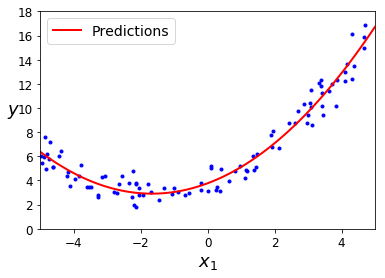
Let’s fit a linear regression model based on X_poly
lin_reg = LinearRegression()
lin_reg.fit(X_poly, y)
lin_reg.intercept_, lin_reg.coef_
(array([3.76999547]), array([[1.0350509 , 0.31123859]]))
X_new=np.linspace(-5, 5, 100).reshape(100, 1)
X_new_poly = poly_features.transform(X_new)
y_new = lin_reg.predict(X_new_poly)
plt.plot(X, y, "b.")
plt.plot(X_new, y_new, "r-", linewidth=2, label="Predictions")
plt.xlabel("$x_1$", fontsize=18)
plt.ylabel("$y$", rotation=0, fontsize=18)
plt.legend(loc="upper left", fontsize=14)
plt.axis([-5, 5, 0, 18])
plt.show()
References
Hands-On Machine Learning with Scikit-Learn and TensorFlow: Concepts, Tools, and Techniques to Build Intelligent Systems