Learning Curves

Learning Curves 24 Mar 2019

In this notebook, we will show how learning curves behaves as a function of the training set size for models with high bias and high variance.

Setup

This cell contains code for referring the common imports that we will be using through this notebook.

# Common imports
import numpy as np
import os

# to make this notebook's output stable across runs
np.random.seed(10)

# To plot pretty figures
import matplotlib as mpl
import matplotlib.pyplot as plt
mpl.rc('axes', labelsize=14)
mpl.rc('xtick', labelsize=12)
mpl.rc('ytick', labelsize=12)

Let’s create a simulated data

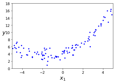
Let’s simulate a quadratic form of our data output.

m = 100
X = 10 * np.random.rand(m, 1) - 5
y = 0.3 * X**2 + X + 4 + np.random.randn(m, 1)

plt.plot(X, y, "b.")
plt.xlabel("$x_1$", fontsize=18)
plt.ylabel("$y$", rotation=0, fontsize=18)
plt.axis([-5, 5, 0, 18])
plt.show()

png

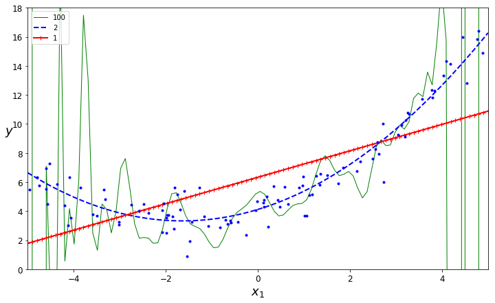
Training three diferent models

A linear model: High Bias
A quadratic model: A Model that fits well
A 100-degree polynomial model: High Variance

from sklearn.linear_model import LinearRegression
from sklearn.preprocessing import PolynomialFeatures
from sklearn.preprocessing import StandardScaler
from sklearn.pipeline import Pipeline

X_new=np.linspace(-5, 5, 100).reshape(100, 1)
plt.figure(figsize=(12,7))

for style, width, degree in (("g-", 1, 100), ("b--", 2, 2), ("r-+", 2, 1)):
    polybig_features = PolynomialFeatures(degree=degree, include_bias=False)
    std_scaler = StandardScaler()
    lin_reg = LinearRegression()
    polynomial_regression = Pipeline([
            ("poly_features", polybig_features),
            ("std_scaler", std_scaler),
            ("lin_reg", lin_reg),
        ])
    polynomial_regression.fit(X, y)
    y_newbig = polynomial_regression.predict(X_new)
    plt.plot(X_new, y_newbig, style, label=str(degree), linewidth=width)

plt.plot(X, y, "b.", linewidth=3)
plt.legend(loc="upper left")
plt.xlabel("$x_1$", fontsize=18)
plt.ylabel("$y$", rotation=0, fontsize=18)
plt.axis([-5, 5, 0, 18])
plt.show()

png

Learning Curves

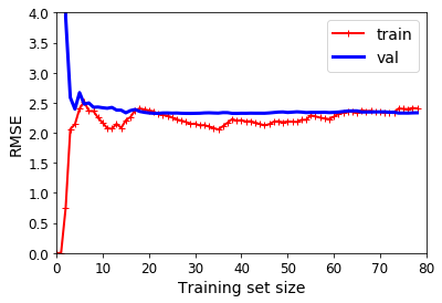
First, let’s plot the learning curve for linear model (high bias). For that goal, we will split the data into training and validation dataset. To plot the learning curve as a function of the training set size, 80 linear models have been trained. The performance (RMSE) is measured for each one of these 80 linear models using the entire validation set.

from sklearn.metrics import mean_squared_error
from sklearn.model_selection import train_test_split

def plot_learning_curves(model, X, y):
    X_train, X_val, y_train, y_val = train_test_split(
                        X, y, test_size=0.2, random_state=11)
    train_errors, val_errors = [], []
    for m in range(1, len(X_train)):
        model.fit(X_train[:m], y_train[:m])
        y_train_predict = model.predict(X_train[:m])
        y_val_predict = model.predict(X_val)
        train_errors.append(mean_squared_error(y_train[:m], y_train_predict))
        val_errors.append(mean_squared_error(y_val, y_val_predict))

    plt.plot(np.sqrt(train_errors), "r-+", linewidth=2, label="train")
    plt.plot(np.sqrt(val_errors), "b-", linewidth=3, label="val")
    plt.legend(loc="upper right", fontsize=14)   
    plt.xlabel("Training set size", fontsize=14) 
    plt.ylabel("RMSE", fontsize=14)              

lin_reg = LinearRegression()
plot_learning_curves(lin_reg, X, y)
plt.axis([0, 80, 0, 4])                         
plt.show()   

png

As we see in the learning curve of a high bias model, the training performance and validation performance get closer each other with a small set size. We also see that increasing the training set size does not help to improve the performance.

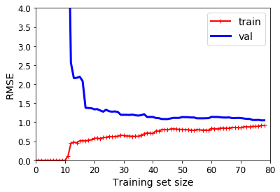
Now, let’s plot the learning curve for a 10-degree polynomial model (high variance). Using a similar approach, we just call the plot learning curve procedure. Similarly, to plot the learning curve as a function of the training set size, 80 polynomial models have been trained. The performance (RMSE) is measured for each one of these 80 linear models using the entire validation set.

from sklearn.pipeline import Pipeline

polynomial_regression = Pipeline([
        ("poly_features", PolynomialFeatures(degree=10, include_bias=False)),
        ("lin_reg", LinearRegression()),
    ])

plot_learning_curves(polynomial_regression, X, y)
plt.axis([0, 80, 0, 4])           
plt.show()   

png

As we see in the learning curve of a high variance model, the training performance and validation performance do not get closer with a small traning set size. But in this case the training size matters, a larger training set size helps that validation performance gets closer to the training performance. It is worth mentioning that this model performs better than the model with high bias.

References

Hands-On Machine Learning with Scikit-Learn and TensorFlow: Concepts, Tools, and Techniques to Build Intelligent Systems